Artificial Source Objects

To generate synthetic images, ArtPop “observes” Source objects. In essence, Source objects are containers that hold the xy pixel positions and stellar mags of the artificial stellar population. As we showed in the Building Stellar Populations and Sampling Spatial Distributions tutorials, ArtPop has the capability to generate these parameters, but you can generate them in any way you want (i.e., independently from ArtPop). You just need to make sure to create xy and mags in the correct format to initialize the Source.

Note: To generate MIST synthetic photometry using ArtPop, MIST isochrone grids are required. The first time you use a MIST grid, ArtPop will download it and save it to your MIST_PATH. If this environment variable is not set, the grid(s) will be saved in ~/.artpop/mist.

# Third-party imports
import numpy as np
import matplotlib.pyplot as plt
from astropy import units as u

# Project import
import artpop

# artpop's matplotlib style
plt.style.use(artpop.mpl_style)

# use this random state for reproducibility
rng = np.random.RandomState(9)

Building a Source Object

In this first example, we will show you how to build a Source object from scratch. We’ll assume a uniform distribution of stars at fixed surface brightness. We start by calculating the mean stellar magnitude of an SSP using the MISTIsochrone class:

iso = artpop.MISTIsochrone(
    log_age = 9,          # log of age in years
    feh = -1,             # metallicity [Fe/H]
    phot_system = 'LSST', # photometric system(s)
)

# normalize the IMF by number
mean_mag = iso.ssp_mag('LSST_i', norm_type='number')

Next we use the constant_sb_stars_per_pix function to calculate the number of stars per pixel this population would have for a given surface brightness and distance (let’s put the population at 10 Mpc):

distance = 10 * u.Mpc
pixel_scale = 0.2

num_stars_per_pix = artpop.constant_sb_stars_per_pix(
    sb = 24,                  # surface brightness
    mean_mag = mean_mag,      # mean stellar magnitude
    distance = distance,      # distance to system
    pixel_scale = pixel_scale # pixel scale in arcsec/pixel
)
print(f'number of stars per pixel = {num_stars_per_pix:.2f}')

number of stars per pixel = 494.43

Let’s say we intend to create an artificial image that is 101 pixels on a side. Then we can calculate the number of pixels, and hence number of stars, in our image.

xy_dim = (101, 101)
num_stars = int(np.multiply(*xy_dim) * num_stars_per_pix)
print(f'number of stars = {num_stars:.0e}')

number of stars = 5e+06

Putting the pieces together, we sample num_stars stellar magnitudes and positions to build our Source object:

# build SSP with num_stars stars
ssp = artpop.SSP(
    isochrone = iso,       # isochrone object
    num_stars = num_stars, # number of stars
    imf = 'kroupa',        # default imf
    distance = distance,   # distance to system
    random_state = rng,    # random state for reproducibility
)

# sample num_stars positions in a uniform grid
xy = np.vstack([rng.uniform(0, xy_dim[0], num_stars),
                rng.uniform(0, xy_dim[1], num_stars)]).T

# create the artificial source
src = artpop.Source(xy, ssp.mag_table, xy_dim)

Note ssp has an attribute called mag_table, which is an astropy table with stellar magnitudes in the given photometric system(s), which is passed as an argument to Source and stored as the mags attribute:

# here are the first 10 rows of the table
# each row corresponds to a single star
src.mags[:10]

Table length=10

LSST_u	LSST_g	LSST_r	LSST_i	LSST_z	LSST_y
float64	float64	float64	float64	float64	float64
47.59355757863038	44.33005922548976	42.78243436679926	41.89141485523699	41.467133437135075	41.25933819275674
43.672879564444045	41.22745392661895	39.96531947084012	39.4238879315009	39.16631172603568	39.01244589273298
43.702311666073996	41.25436463467862	39.99056155533645	39.44808389608072	39.19001162581168	39.0358924533673
46.29019385112325	43.421740839257744	41.967908643812656	41.234118360975835	40.884716609196985	40.69384323226573
46.201714598907216	43.35640814961155	41.908833116665	41.18516833149769	40.84014555128736	40.65018191045182
45.39264915593941	42.721913816438494	41.334921530569915	40.69067124092121	40.38236025543267	40.20509055510217
44.10579588525191	41.62031671900799	40.332753796445324	39.77460605482946	39.50910028277801	39.35137020065203
45.17359479981009	42.5389985675621	41.1691338679598	40.54222253642945	40.24240241939206	40.0694116529263
46.82327513973055	43.804974275055656	42.31210839002173	41.51577945269061	41.13666009211553	40.939627726304245
44.536376030908954	41.9964770290303	40.677215855851706	40.09522142938339	39.81805085427266	39.655400968864015

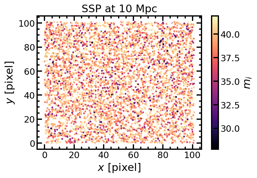
The src object contains all the information about the source that we need to simulate an observation, which is described in the Making Artificial Images tutorial.

Here’s a look at the positions and \(i\)-band magnitudes of a random subset of the stars in src:

idx = rng.choice(np.arange(src.num_stars), 5000, replace=False)
plt.scatter(src.x[idx], src.y[idx], s=4,
            c=src.mags['LSST_i'][idx], cmap='magma')

cbar = plt.colorbar()
cbar.ax.set_ylabel('$m_i$')
plt.xlabel('$x$ [pixel]')
plt.ylabel('$y$ [pixel]')
plt.title(f'SSP at {distance:.0f}')
plt.minorticks_on();

As a sanity check, we can calculate the surface brightness of the population:

total_flux = (10**(-0.4 * src.mags['LSST_i'])).sum()
area = np.multiply(*xy_dim) * pixel_scale**2
sb = -2.5 * np.log10(total_flux / area)
print(f'SB = {sb:.2f} mag / arcsec^2')

SB = 24.00 mag / arcsec^2

Helper SSP Source Objects

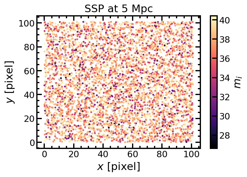
For convenience, ArtPop provides objects for generating SSP + spatial distribution combinations. Here we generate an SSP with a uniform spatial distribution, similar to above, using the MISTUniformSSP helper class:

# let's put the population at 5 Mpc
distance = 5 * u.Mpc

# create ssp distributed uniformly in space
src_uniform = artpop.MISTUniformSSP(
    log_age = 9,          # log of age in years
    feh = -1,             # metallicity [Fe/H]
    phot_system = 'LSST', # photometric system(s)
    distance = distance,  # distance to system
    xy_dim = 101,         # image dimension (101, 101)
    pixel_scale = 0.2,    # pixel scale in arcsec / pixel
    sb = 24,              # surface brightness (SB)
    sb_band='LSST_i',     # bandpass to calculate the SB
    random_state = rng,   # random state for reproducibility
)

# plot positions with symbols colored by i-band mags
idx = rng.choice(np.arange(src_uniform.num_stars), 5000, replace=False)
plt.scatter(src_uniform.x[idx], src_uniform.y[idx], s=4,
            c=src_uniform.mags['LSST_i'][idx], cmap='magma')

cbar = plt.colorbar()
cbar.ax.set_ylabel('$m_i$')
plt.xlabel('$x$ [pixel]')
plt.ylabel('$y$ [pixel]')
plt.title(f'SSP at {distance:.0f}')
plt.minorticks_on();

Composite Sources

Similar to creating composite stellar populations, composite Source objects are created intuitively using the + operator. Here we’ll use MISTPlummerSSP to create an SSP with a Plummer spatial distribution and add it to the uniformly distributed population we created above:

# create ssp distributed uniformly in space
src_plummer = artpop.MISTPlummerSSP(
    log_age = 10.1,           # log of age in years
    feh = -1.5,               # metallicity [Fe/H]
    scale_radius = 20 * u.pc, # effective radius
    num_stars = 5e5,          # number of stars
    phot_system = 'LSST',     # photometric system(s)
    distance = distance,      # distance to system
    xy_dim = 101,             # image dimension (101, 101)
    pixel_scale = 0.2,        # pixel scale in arcsec / pixel
    random_state = rng,       # random state for reproducibility
)

# add sources together
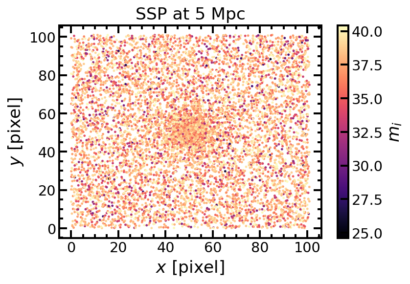
composite_src = src_uniform + src_plummer

# plot positions with symbols colored by i-band mags
idx = rng.choice(np.arange(composite_src.num_stars), int(1e4), replace=False)
plt.scatter(composite_src.x[idx], composite_src.y[idx], s=2,
            c=composite_src.mags['LSST_i'][idx], cmap='magma')

cbar = plt.colorbar()
cbar.ax.set_ylabel('$m_i$')
plt.xlabel('$x$ [pixel]')
plt.ylabel('$y$ [pixel]')
plt.title(f'SSP at {distance:.0f}')
plt.minorticks_on();

WARNING: 2656 stars outside the image